Fair Decathlon Model. Part 10: Ten Events. One Decathlon. One Clock. (0)

FAIR DECATHLON MODEL

PART X

Ten Events. One Decathlon. One Clock.

A final thought experiment after the Fair Decathlon Model

Rafal Snoch   |   for Decathlon2000.com   |   August 2026

After nine parts

The Fair Decathlon Model has reached the point at which its original job can be considered finished. The upper calibration was rebuilt across forty seasons, the formulas were tested outside their anchors, the lower population was examined in detail, the ten event distributions were pushed deep into the lower tail, and Part VIII finally audited the zero-point parameter B event by event. Part IX then asked the question underneath all of that mathematics: what should a decathlon scoring table actually measure?

If the answer is still a traditional decathlon scored in points, FDM-B is ready for that job. Nothing in this final part is needed to make FDM-B complete. A reader who prefers the familiar structure - ten performances, ten point scores, one total - can stop there.

One old problem remains, however, no matter how good the point table becomes. The 1500 metres ends. The athletes cross the line. Then the stadium still has to wait: the times must be confirmed, the 1500-metre points calculated, the totals added, and only then does the final order become certain. The last race is the final event, but it is not quite the final classification.

Does decathlon need points?

The question is deliberately narrow. It does not ask whether points are useless. They are extremely useful for personal bests, qualification standards, records and historical comparison. It asks only this: does the internal competition itself need to be expressed in points, or does it only need a coherent way to exchange advantage between ten different events?

2018: two questions that never met

On 3 June 2018, Richard Crawford published Are the Decathlon Tables Fair? His definition of fairness was differential. For athletes of comparable ability, an improvement from one percentile to another should create a comparable change in the combined-event score regardless of the event. Importantly, Crawford did not say that the same exchange rate had to apply at every performance level. The 30th-to-40th percentile step could be different from the 50th-to-60th step. The essential question was whether comparable sporting improvements were exchanged comparably across events.

Later that year, the IAAF Council approved the introduction of the Gundersen method for the final races of the combined events at the 2020 World U20 Championships in Nairobi. The idea was visually simple: after the earlier events, the points gaps would be converted into time gaps for the final race, so that the order across the finish line could become the final classification.

The two projects were looking at different halves of the same problem. Crawford examined measurement without changing the visible competition. The Gundersen proposal tried to change the visible competition without rebuilding the measurement underneath it. They went separate ways.

Crawford-Gundersen asks what happens if those unfinished questions are joined. First establish a coherent exchange relationship between the events. Then let that same relationship become the pursuit itself.

The name "Crawford-Gundersen" is descriptive, not an attribution of authorship or endorsement. Crawford supplied the analytical fairness question; the Gundersen idea supplies the pursuit logic. The combination proposed here is a separate thought experiment.

Why the earlier Gundersen idea was not enough

The 2018 approach was effectively a presentation layer attached to the official scoring tables. The first nine events would still be valued by nine progressive power functions. Only after the ninth event would the resulting point gap be converted linearly into seconds for the 1500 metres.

That can produce an exciting finish, but it creates a hybrid. For nine events the exchange rate between metres, seconds and points changes with performance level. At the last moment, that nonlinear point difference is translated into one linear time handicap. The pursuit becomes readable, but the underlying competition never receives a single common unit.

The proposal here is different. It uses one linear time currency from the first 100 metres to the finish of the 1500 metres. The question is therefore no longer "how many seconds should one point be worth at the end?" It becomes "how many seconds should a tenth of a second, a centimetre or a metre be worth throughout the decathlon?"

A deliberate simplification

This is the point at which the proposal gives up something on purpose. FDM-B remains the more nuanced mathematical model. Its power functions allow the exchange value of a metre or second to change across the performance scale, and that curvature may describe the extremes more faithfully than a straight line.

Crawford-Gundersen does not claim the relationship between performance and sporting value is globally linear, or that a fixed exchange rate is mathematically truer than a power function. It asks whether a constant rate can be a sufficiently good sporting approximation in return for a large practical gain: a competition that athletes, coaches, commentators and spectators can read directly in one unit.

The data collected during FDM make that compromise less arbitrary than it would have been at the beginning of the project. In Part III, the 10th- and 140th-ranked forty-season mean performances were used as the two fixed upper anchors, while the 75th-ranked performances were left as an independent middle control. The model reproduced that unused middle level very closely. Rank 75 is also exactly halfway between ranks 10 and 140 in rank distance: 65 places in either direction. That does not prove linearity, but it shows that the broad exchange geometry across the elite calibration span is smooth and stable rather than fragile.

Part VII then moved the experiment far away from the elite. In a 10,720-performance lower database containing no complete decathlon of 7000 points or more, independently ranked event distributions remained extremely compact through R5200 and were still largely coherent at R7800. When those R7800 marks were located in the full 27,741-performance master, nine events lay at roughly the 89th percentile of their distributions and the 1500 metres at about the 87th. Strong divergence became dominant only deeper in the tail.

Again, this is not proof that one immutable straight line governs every level of the sport. It is narrower evidence: through most of the observed distribution, the ten events preserve stable enough relationships that a fixed exchange rate is not contradicted by the data. For a system designed to gain live readability, that provides a reasonable empirical basis for simplification.

The current scale is calibrated for the senior men's decathlon with standard senior hurdles and implements. Junior, youth or masters versions would require their own calibration wherever the event specifications change.

One currency: 1500-metre seconds

The common currency is the second of the 1500 metres. The forty-season reference data give a mean of 4:22.09 at rank 10 and 5:00.46 at rank 140 — a difference of 38.37 seconds. Crawford-Gundersen treats the corresponding 10th-to-140th span in every other event as the same difference in sporting level.

In the discus, that span is 48.18–37.04 m, or 11.14 m. Dividing 38.37 by 11.14 gives 3.44 CG seconds per metre. In the 100 m, the span is 10.69–11.45 s, or 0.76 s, which gives 50.49 CG seconds per second. The same calculation produces the exchange rate for every event.

The rates are defined to two decimal places, and all calculations below use the displayed values.

A fixed reference for the clock

Exchange rates are enough to determine gaps between athletes, but an absolute CG result also needs an origin. For the first nine events, this proposal uses a fixed performance profile worth 912.6 continuous FDM-B points in each event. The number is chosen because ten times 912.6 equals 9126, Kevin Mayer's official world-record total. It places the clock on a familiar elite scale without making Mayer's actual event profile the reference.

The final FDM-B coefficients from Part VIII give the rounded reference marks shown in Table 1: 10.60 for the 100 metres, 7.71 m in the long jump, 15.98 m in the shot put, 2.12 m in the high jump, 47.59 for 400 metres, 14.02 in the hurdles, 49.63 m in the discus, 5.20 m in the pole vault and 68.10 m in the javelin.

Table 1. Crawford-Gundersen exchange rates and the fixed FDM-B reference profile

Reference spans: 40-season mean marks at ranks 10 and 140 from Part III.

After each of the first nine events, the calculation is ordinary arithmetic. A 10.50 100 metres is 0.10 seconds faster than the 10.60 reference, so it earns a 5.05-second gain. A 50.63 m discus is 1.00 m beyond the 49.63 reference, so it earns a 3.44-second gain. A mark worse than the reference adds time instead. Gains are shown as negative balance; losses as positive balance.

The same exchange rate applies at every level. A 15-metre difference in the javelin is worth 34.20 CG seconds whether the marks are 75 m and 60 m or 30 m and 15 m. The absolute quality of the two pairs is obviously different. The rule for exchanging the difference is not.

What the scoreboard shows

A live Crawford-Gundersen scoreboard needs only two time columns beyond the ordinary event result. The first is the athlete's cumulative balance against the fixed reference profile. The second is the gap to the current leader.

Illustrative display only. The gap-to-leader column is always non-negative.

This creates two stories at once. The reference balance gives an absolute performance trajectory that can later become a personal best, meeting record or historical result. The leader gap tells the competition story. Before the 1500 metres, that second column becomes the starting handicap without any additional conversion.

A coach can therefore read the race before it happens. If an athlete is 12 seconds behind after the javelin and is normally 20 seconds faster over 1500 metres than the leader, the problem is visible immediately. No one needs to translate a point gap into an approximate target time after nine events. The gap is already a time.

No zero-point cliff

Linearity has another consequence. Crawford-Gundersen does not need B, the parameter that tells a power function where positive scoring ends. There is no mathematical cliff at which a very poor but valid performance suddenly becomes indistinguishable from an even poorer valid performance.

That matters most at the bottom of the scale. Part IX used the 1500 metres to expose the difference. Under FDM-B, 480 seconds is the zero-point boundary. A completed 8:01 and a non-finish both lie beyond the positive scoring region, but they are not the same sporting act. One athlete completed the decathlon; the other did not.

In CG, a valid 8:01 is simply 481 seconds of actual final-race time. A valid 9:30 is 570 seconds. A valid 9:50 is 590 seconds. The 20-second difference remains a 20-second difference. The system never has to decide that both performances are "zero" and therefore equal.

The same principle applies in the field. A legal throw of 0.50 m would be an extraordinarily weak result, but it would still carry information. It would create a very large time loss. It would not disappear. Weak performance and missing performance are different categories.

Ten valid events - or no decathlon result

That distinction makes the completion rule simpler rather than softer. Under this proposal, an official Crawford-Gundersen result requires ten valid event performances and a finish in the 1500 metres. If an athlete records no valid result in event n, he does not start event n+1 or any later event.

The closest analogy is a stage race. A rider who does not finish stage five of the Tour de France does not return for stage six and cannot reappear on the Champs-Elysees for the final stage. A decathlete who has no valid hurdles result has no value to compare with the hurdles reference. There is nothing to carry forward into the discus. A runner who does not finish the 1500 metres has no final time to complete the ten-event result.

There is no substitute mark, no artificial time penalty and no zero-point replacement. A missing event is not an extremely poor performance. It is a missing part of the decathlon.

This also removes a strange possibility that exists in conventional point scoring. An athlete with a sufficiently large lead after nine events can, in principle, start the 1500 metres, fail to finish, receive zero points for the race and still retain the highest ten-event point total. In Crawford-Gundersen, a large lead can buy a very slow and very safe 1500 metres. It cannot buy permission not to finish it.

You may win an event. To win the decathlon, you must complete the whole race.

The 1500 metres becomes the real final

After the javelin, nothing new has to be calculated. The accumulated CG balances already contain the first nine events. The athlete with the lowest balance starts first. Every other athlete starts later by exactly the difference between his balance and the leader's.

Suppose Athlete A leads with a balance of -12.00 seconds and Athlete B has +3.00. B starts 15.00 seconds later. If A then runs 4:40.00 and B runs 4:24.00, B gains 16 seconds in the final race and crosses the finish line one second ahead. The finish order is the decathlon order because the track has physically consumed the entire previous gap.

The clock can preserve the absolute result at the same time. In that example, the leader's clock begins at -0:12.00 when A is released. B's start gate opens when the clock reaches +0:03.00. At the finish, A's displayed CG result is 4:28.00 and B's is 4:27.00. The number on the clock is not a separate race time followed by a calculation. It is the complete decathlon result.

A pilot competition would use electronic release and timing to 0.01-second precision. The exact gate design, start commands and fail-safe procedures are technical questions for testing, but they do not alter the scoring principle.

Want the gold medal? Cross the finish line first.

The geometry problem

A pursuit final creates one problem that ordinary 1500-metre racing does not have. Large starting handicaps can approach the time required for a full lap.

For a simple elite range, take 1500-metre times from 4:10 to 5:00. Those correspond to average 400-metre paces of about 66.7 to 80.0 seconds. A handicap of roughly that size therefore creates the possibility that a leader completes an extra 400 metres and arrives physically beside an athlete who is only just starting or is still a full lap behind in the total pursuit.

If everyone uses the inside lane from the beginning, the oval can create a false meeting. Two athletes may be shoulder to shoulder on the track even though one is approximately 400 metres ahead in the complete decathlon race. That can produce obstruction, accidental pacing or drafting between athletes who have not genuinely caught each other.

Instead of fighting the geometry of the stadium, the Snail course uses it.

The Snail-Crawford-Gundersen course

On the current eight-lane layout, the 1500-metre pursuit begins in the outer two-lane corridor and then moves inward through four successive corridors: lanes 7-8, then 5-6, then 3-4, and finally 1-2. The transitions turn the ordinary oval into a shallow spiral.

The sporting principle is simple. Athletes who are separated only because one has completed an extra loop of the oval remain in different corridors. Athletes who genuinely catch each other in the complete pursuit eventually occupy the same part of the route. Once the catch is real, normal racing interaction is welcome: they can overtake, use each other for pace or fight directly for position.

In other words: you may use the rival whom you have genuinely caught - not a rival whom you meet only because the track loops every 400 metres.

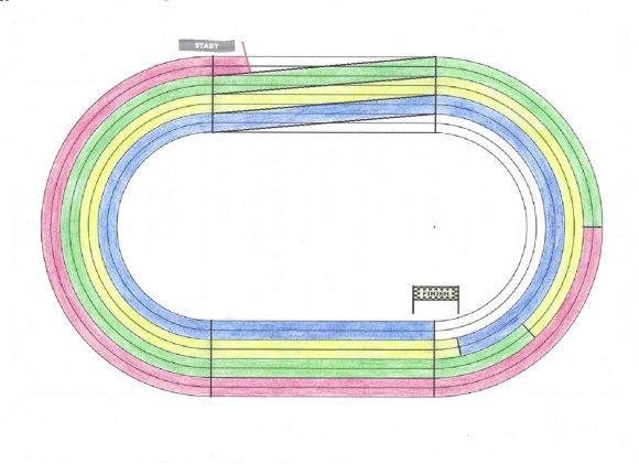
Figure 1. Current calculated eight-lane Snail layout: 7-8 -> 5-6 -> 3-4 -> 1-2. A competition version would still require formal measurement, safety testing and certification.

A nine-lane stadium offers a natural variation: 8-9, then 6-7, then 4-5, and finally the wider 1-3 corridor. The exact start line and transition positions would have to be remeasured for that geometry so that the prescribed route remains exactly 1500 metres.

The Snail is therefore not an ornamental addition to the scoring system. It solves a problem created by the pursuit itself. A real pilot would still have to test transition markings, right-of-way, safe field size and overtaking space. Those are operational questions. The central geometric idea is already clear: use the lanes to keep false lap encounters apart while preserving genuine catches.

What happens to real elite decathlons?

A radical format should at least be tested against performances we already know. The table below shows how the current all-time top 15 would look under Crawford-Gundersen. The purpose is not to prove the system from fifteen performances, but to see whether a linear time scale still recognises the same world-class structure.

Table 2. Crawford-Gundersen recalculation of the supplied all-time OFF top 15

The ranking remains very stable. Kevin Mayer and Ashton Eaton remain first and second; Damian Warner and Roman Šebrle exchange third and fourth. Dan O'Brien and Kyle Garland each rise one place. Of the two OFF ties, Pierce LePage remains seventh while Sander Aae Skotheim falls from joint seventh to tenth, and Jürgen Hingsen remains thirteenth while Bryan Clay moves to fourteenth. The remaining positions are unchanged.

The added FDM column shows something more. CG is not simply OFF expressed in seconds, but neither is it FDM expressed in another unit. FDM ranks Eaton first, Warner second and Mayer third; CG returns Mayer to first, followed by Eaton and Warner. The three systems make some different close judgements, yet the broad elite structure remains remarkably stable. That is exactly what a useful linear approximation should do: simplify the exchange mechanism without erasing the sporting hierarchy.

The table is therefore not a retrospective record list. These performances were achieved under the traditional decathlon format, not under Crawford-Gundersen rules. They are used here only to show what the new scale does to performances we already know. If Crawford-Gundersen were ever contested in practice, its records would begin with the first competition actually held under those rules.

What happens across 27,741 complete decathlons?

The elite table is only a first check. The stronger test is to apply exactly the same fixed exchange rates to the full 27,741-performance master used in Part VII.

Across all 27,741 complete decathlons, the Spearman rank correlation between the FDM-B and CG orderings is 0.99970. The OFF and CG orderings are also very close, at 0.99686. Rank correlation alone does not prove that the underlying power functions are linear. It does show that replacing their curvature with the fixed CG rates changes remarkably little in the ordering of real complete decathlons.

This joins the two kinds of evidence. Part VII showed that the ten event distributions remain coherent through most of the observed scale. The full-master test now shows that a fixed linear translation preserves almost the same whole-decathlon structure. The claim is not that the power functions become straight lines; it is that the linear approximation loses surprisingly little across the range in which real decathlons are performed.

The same data also give the new clock a familiar scale. Using performances within ±50 OFF points of each reference level, the median CG times are:

Table 3. Typical Crawford-Gundersen times at familiar OFF levels

These are population medians, not fixed conversion formulas: two performances with the same OFF total can still produce different CG times because the systems value profiles differently. Even so, the mapping is tight. Around 8000 OFF, the middle half of the sample lies between about 7:33 and 7:45 CG; around 7000, between about 10:39 and 10:54.

What the system gains

The trade is now visible. Crawford-Gundersen gives up some of the curvature and mathematical refinement of FDM-B. In return, it gains a form of transparency that a point table cannot easily provide.

• One exchange language. A metre or second has a fixed CG value that an athlete can learn once and keep throughout his career.
• One live classification. After every event, the leader gap is already expressed in the unit that matters for the final.
• No zero-point loss of resolution. Every valid mark remains distinguishable, however weak.
• One completion rule. Very poor is allowed; missing is not.
• A genuine pursuit. The start gaps after nine events are the actual accumulated gaps, not a presentation conversion added at the end.
• A visible winner. The first athlete across the 1500-metre finish line wins the decathlon.
• One absolute result. The clock at the finish can serve as the athlete's CG personal best, meeting record or historical performance.

None of those advantages proves that CG should replace the traditional decathlon. They explain why the simplification may be worth testing. FDM spent nine parts asking how to make the exchange between events more defensible. Crawford-Gundersen asks whether, once that exchange is understood, it can also be made visible.

FDM-B and Crawford-Gundersen

The two systems do not have to compete for the same role. FDM-B is the completed scoring model for the traditional point-based decathlon. It keeps the power-function structure, retains a carefully audited lower boundary in each event and tries to describe the full scoring scale with more mathematical nuance.

Crawford-Gundersen is a different layer of thought. It borrows the empirical relationships established by FDM, replaces variable exchange rates with fixed local approximations, and spends the mathematical precision it gives up on readability, continuity and a true pursuit finish.

If the traditional format is the goal, use FDM-B. If the question is whether the decathlon can become easier to understand live without abandoning the internal relationships discovered in the data, Crawford-Gundersen is the experiment to try.

That is why Part X is not a correction to the first nine parts. It is what becomes possible after them.

One clock

A scoring table normally disappears behind the competition. Athletes produce marks, the table converts them, and the audience receives a total. Crawford-Gundersen tries to reverse that relationship. The exchange mechanism becomes visible as time, the accumulated competition becomes a pursuit, and the final clock carries the whole decathlon across the finish line.

The proposal may ultimately prove too radical, too difficult to stage, or simply less attractive than the tradition it challenges. That is exactly what a pilot competition would be for. But the question is now concrete enough to test rather than merely imagine.

Can ten unlike events be connected by one stable exchange currency? Part VII suggested that, through most of the observed scale, the relationships were stable enough to try. The full 27,741-performance recalculation now shows that the fixed CG rates preserve the FDM-B ranking structure almost exactly (Spearman rho = 0.99970). Can that currency become a pursuit without creating false lap encounters? The Snail uses the geometry of the track to try to solve that problem. Can the winner be known at the finish line without sacrificing an absolute historical result? One clock can do both.

Ten Events. One Decathlon. One Clock.

Acknowledgements

This ten-part project could not have developed in the same way without Decathlon2000.com. My thanks to Janek for giving the series a home, for publishing a project that changed direction as the data demanded, and for reading the argument closely enough to understand not only the formulas but the questions underneath them.

I also owe a particular intellectual debt to Richard Crawford. His 2018 work did not provide the FDM formulas, and Crawford-Gundersen should not be read as his proposal. What it did provide was a durable way of asking the fairness question — and, as this project developed, considerably more than that. Crawford’s Table 1 turned out to contain a remarkably rich description of the decathlon population. Before my own lower-level database was large enough to speak clearly, its cohort medians already allowed several population trends to be estimated; many of those estimates were later reproduced by the expanded FDM data. In that sense, Crawford’s work did not merely inspire the question. It repeatedly helped point the investigation in the right direction.

Any errors in the calculations, interpretations or competition design presented here are mine.

Sources and notes

• Richard Crawford, Are the Decathlon Tables Fair?, research manuscript dated 3 June 2018.

• Richard Crawford, The Principles Underlying the Tables.

• IAAF Council decisions, 2018, approving the introduction of the Gundersen method for the final races of the combined events at the 2020 World U20 Championships; further development discussed by the IAAF Council in 2019.

• Fair Decathlon Model, Part III: Forty Seasons, Cleaner Data, and Wider Calibration.

• Fair Decathlon Model, Part VII: Can Decathlon Calibrate Itself?

• Fair Decathlon Model, Part VIII: Where Should Zero Points Begin?

• Fair Decathlon Model, Part IX: Ten Events. One Decathlon.

• FDM master database: 27,741 complete decathlons used for the full-population Crawford-Gundersen test in this part.

• All-time top-15 marks used in Table 2: Decathlon2000.com list supplied for this study.

Rafał Snoch for Decathlon 2000